Developing Scale Inhibitor Dosage Models
Robert J. Ferguson
French Creek Software, Inc.
Kimberton and Hares Hill Road, Box 684
Kimberton, Pennsylvania 19442 U.S.A.
Presented at WaterTech '92, Houston, Texas
NACE EUROPE '93, Sandefjord, Norway
Published in Industrial Water Treatment Magazine
Abstract
Feeding the minimum effective inhibitor dosage can
reduce operating costs for chemical treatment, minimize treatment chemical
discharge to the environment, and in some cases, prevent underfeed
of a scale inhibitor. Common sense indicates that the same scale inhibitor
dosage is not required for all waters and systems. One size does not fit
all. Water treatment companies have capitalized on this general concept
since the introduction of first computerized water chemistry evaluation
and treatment recommendation systems in the 70's.(1,2,3)
Dosage models have been developed by the industry for scale control in
applications ranging from long residence time open recirculating cooling
tower systems, to the ultra low treatment levels required in very short
residence time once through utility surface condenser cooling systems.
This paper discusses the parameters critical to developing an effective
dosage modulation model for scale inhibitors from laboratory data, field
data, or a combination of both. The paper draws upon the concept of induction
time as a basis for the mathematical models used to develop predictive
models from actual data. The models are based upon the concept that threshold
effect inhibitors do not prevent scale formation, they only delay the inevitable.
The models are in agreement with current theories and treat scale inhibitors
as agents which extend the induction time before crystal formation and/or
growth on existing active sites occurs in the case of calcium carbonate,
and as dispersants which control particle size in the case of calcium phosphate.
The models predict the dosage required to inhibit deposition until the
treated water has passed through a cooling system. This delay can vary
from 3 to 15 seconds in a large volume once through condenser cooling system,
to days in open recirculating cooling systems.
Thermodynamic driving forces and system operating conditions are used by
the models to describe the kinetics of scale formation, growth, and the
impact of inhibitors upon induction time.
Similar models to those discussed have been used successfully to optimize
scale inhibitor treatments in once through utility cooling systems and
open recirculating cooling systems since the late 70's.
Introduction
The models described in this paper were developed from a combination
of field observations, common sense, and laboratory data. Model development
began in the early 1970's. At this time, utilities using manmade impounded
lakes as a source for condenser cooling water were beginning to develop
condenser scale problems. The lakes were originally filled with water of
a low scale potential. The heat load from condenser cooling, and the lack
of blowdown, caused the lakes to concentrate with time. Calcium carbonate
scale became an economically significant problem after several years of
operation. Deration was encountered due to high condenser back pressure
in addition to the heat rate penalty associated with increased back pressure
due to condenser deposits. Treatment with scale control agents would have
cost more than the problem if treatment were implemented using the once
through cooling technologies of the time. New technology was needed if
the treatment of these systems for scale control was to be economically
feasible. Dosage optimization studies were conducted to determine if ultra
low dosages, on the close order of 0.001 to 0.2 mg/l active, could effectively
prevent calcium carbonate scale.
The initial studies were conducted using well instrumented test heat exchangers.
Tests were run in parallel. One exchanger was treated at a high level to
assure that scale would be controlled. The parallel exchanger remained
untreated. Fouling factors were monitored continuously on the exchangers.
Fouling could be measured a day or two prior to the formation of a visible
deposit.
The time required for measurable deposit formation was noted. This time
was used to determine the minimum time between dosage reductions during
the dosage optimization studies. Dosage reductions were made after a minimum
of two of these time periods had elapsed.
It was observed that ultra low dosages were effective in preventing scale
formation in the short residence time condensers. The cooling water was
present in the condensers for less than 10 seconds in all of the systems
evaluated. Models were developed based upon the initial studies at seven
(7) locations. The once through cooling system data was later expanded
to longer residence time open recirculating (cooling tower) systems. Laboratory
studies filled data gaps.
During the evaluation of the data it was found that several parameters
were critical to dosage: time, temperature,
and the degree of supersaturation. System cleanliness was
also found to be important. This paper discusses the models and their practical
application to cooling water scale control. The method outlined in this
paper has been used to develop models of minimum effective inhibitor dosages
from laboratory data, field data, and combinations of both. The models
provide a natural path for bringing research data into the practical arena
of the operating engineer or water chemist.
The use of the models is described in case history format, after a brief
description of the impact of individual parameters upon the minimum effective
scale inhibitor dosages.
Induction Time: The Key To The Models
Reactions do not occur instantaneously. A time delay occurs once all
of the reactants have been added together. They must come together in the
reaction media to allow the reaction to happen. The time required before
a reaction begins is termed the induction time.
Thermodynamic evaluations of a cooling water scale potential predict what
will happen if a water is allowed to sit undisturbed under the same conditions
for an infinite period of time. Even simplified indices of scale potential
such as the Langelier saturation index can be interpreted in terms of the
kinetics of scale formation. For example, calcium carbonate scale formation
would not be expected in an operating system when the Langelier saturation
index for the system where 0.1 to 0.2 . The driving force for scale formation
is too low for scale formation to occur in finite, practical cooling system
residence times. Scale would be expected if the same system operated with
a Langelier saturation index of 2.8 . The driving force for scale formation
in this case is high enough, and induction time short enough, to allow
scale formation in even the longest holding time index cooling systems.
Induction time has been modeled for economically important crystals such
as sucrose. Models follow a formula similar to equation
_________________________________________1
EQUATION 1_______ Induction Time =
_____________________
________________________________k
[Saturation Level 1]P1
where
Induction Time is the time before crystal formation and growth
occurs;
k is a temperature dependent constant;
Saturation Level is the degree of supersaturation;
P is the critical number of molecules in a cluster prior to phase
change.
Gill and his associates demonstrated that commercially available scale
inhibitors extend the induction time for calcium carbonate scale(4).
Their paper points out several critical parameters which impact the induction
time prior to crystal growth:
The degree of supersaturation.
The temperature.
The presence of active sites upon which growth can occur.
The inhibitor level.
Gill's study used saturation level as the thermodynamic driving force
for scale growth. Saturation level calculations performed using a computerized
ion pairing method eliminate most of the assumptions inherent in simplified
indices(5). They account for common ion effects which
can increase the apparent solubility of a scale forming specie such as
calcium carbonate. Driving forces for scale formation calculated using
the ion pairing method are transportable between systems because they base
their calculations upon free ion concentrations rather than the total analytical
values. This is the heart of the ion pairing, or ion association method,
which subtracts ion pairs (e.g. CaSO4, CaHCO3)
from the total analytical value to estimate the free ion present and available
to react in forming seed crystals, or in driving growth on existing substrates.
The remainder of this paper uses ion association model saturation levels
for the driving force for scale formation. Table 1 provides a working definition
of the term saturation level for calcium carbonate and tricalcium phosphate.
Critical Parameters
The parameters contributing to equation 1 are included in the basic
relationships used for inhibitor dosage modeling. Major data values required
include the time period during which scale formation must be prevented,
the degree of supersaturation which is the driving force which must
be overcome, the temperature at which the inhibitor must function,
and the pH of the cooling water. The surface area of active sites
also impacts the dosage requirement.
These parameters have the following impacts upon dosage:
Time The time selected is the residence time the inhibited
water will be in the cooling system. The inhibitor must prevent scale formation
or growth until the water has passed through the system and been discharged.
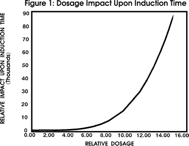
Figure 1 profiles the impact of induction time upon
dosage with all other parameters held constant.
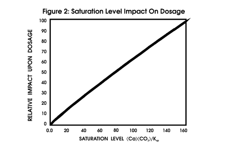
Degree of Supersaturation An ion association model saturation
level is the driving force for the model outlined in this paper, although
other, similar driving forces have been used. Calculation of driving force
requires a complete water analysis, and the temperature at which the driving
force should be calculated. Figure
2 profiles the impact of saturation level upon dosage, all other parameters
being constant.
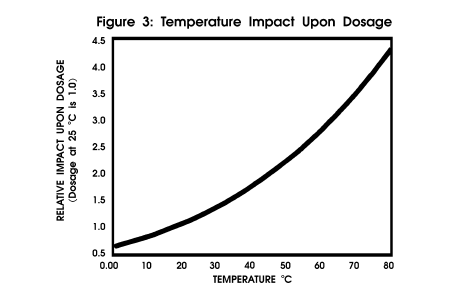
Temperature Temperature affects the rate constant for the
induction time relationship. As in any kinetic formula, the temperature
has a great impact upon the collision frequency of the reactants. This
temperature effect is independent of the effect of temperature upon saturation
level calculations. Figure 3
profiles the impact of temperature upon dosage with other critical parameters
held constant.
pH pH affects the saturation level calculations, but it also
may affect the dissociation state and stereochemistry of the inhibitors(8).
Inhibitor effectiveness can be a function of pH due to its impact upon
the charge and shape of an inhibitor molecule. This effect may not always
be significant in the pH range of interest (e.g. 6.5 to 9.5 for cooling
water).
Active sites It is easier to keep a clean system clean than
it is to keep a dirty system from getting dirtier. This rule of thumb may
well be related to the number of active sites for growth in a system. When
active sites are available, scale forming species can skip the crystal
formation stage and proceed directly to crystal growth.
Other factors can impact dosage such as suspended solids in the water.
Suspended solids can act as sources of active sites, and can reduce the
effective inhibitor concentration in a water by adsorption of the inhibitor.
These other factors are not taken into account in the models in this paper.
Table 2 summarizes the factors
critical to dosage modeling, and their impact upon dosage.
Data Base
The dosage models used as examples in this paper were developed from
data collected in field studies(6), laboratory studies,
published data, or a combination of these sources.
Examples in this paper include data from sidestream evaluation of the minimum
effective dosages in utility surface condensers.(6,7)
In these studies, two parallel fouling probes were used to develop estimates
of the minimum effective dosages for the phosphonates aminotrismethylene
phosphonic acid (AMP), 1,1hydroxy ethylidene diphosphonic acid (HEDP),
and polyacrylic acid (PAA). One probe was overtreated at a level where
no calcium carbonate deposition would be anticipated. The parallel probe
was not treated, and the time required for a measurable deposit to form
determined. This was deemed the minimum period between dosage adjustments
for the test. (Note: A minimum test duration of twice the time required
for fouling was allowed to pass between dosage adjustments). Dosages were
decreased until failure, as indicated by a measurable deposit formation.
Inhibitor dosages were then decreased to the minimum effective level on
the condenser cooling systems to confirm that the dosages did indeed prevent
scale. Condenser cleanliness was monitored by heat transfer. This work
was done in the late 70's when subppm treatment levels and ultra low
dosages were just beginning to be used in utility once through cooling
system scale control programs.
A dosage model is only as good as the data from which it is derived. The
most generally applicable models include data points over the anticipated
ranges for critical parameters. For example, a model developed using data
in the temperature range of 30 to 40 ºC might be totally useless in
predicting a dosage for a system operating at 70 ºC.
Models should be derived from data over the range of water chemistry anticipated
as well as over the range of saturation level anticipated. If a calcium
carbonate scale inhibitor model will be used in waters ranging from a calcium
level of 40 ppm to over 1000 ppm, this range should be covered from laboratory
and/or field sources. The saturation level range anticipated should also
be bracketed (e.g. 1.0 to 250 saturation level for calcite).
Although field data is the source of choice, field conditions can rarely
be adjusted to cover the temperature, pH, time, and water chemistry ranges
desired. The use of static laboratory tests designed to elucidate the variation
of dosage with any of the parameters can be used to supplement field data.
Field data, although desirable, is not always necessary for the development
of a preliminary correlation. As demonstrated in the calcium phosphate
deposit control example, dosages predicted by laboratory tests can be directly
applicable to field conditions. Each model developed should be compared
to field results to assure that a correlation exists between the test data,
the model, and actual field results.
Development Of A Model
A modified version of Equation 1 provided the basis for model correlation.
Dosage was added as a factor to the equation on the right side to
produce Equation 2.
____________________________________________________DosageM
Equation 2 ______________________Induction
Time = ________________________
______________________________________________k'[Saturation
level 1]P1
The temperature dependent rate constant k' was found to
correlate with the Arrhenius relationship (Equation 3).
Equation 3 ______________________k'
= A eEa/RT
Saturation levels were calculated from water analysis input using
a computerized ion association model. The time used for the correlation
is the time to failure in laboratory tests, the residence time in a heated
state for utility once through cooling systems, and the holding time index
in open recirculating cooling systems.
Equation 2 was rearranged to solve for dosage in the first order. Regression
analysis was used to estimate the coefficients.
Field Correlation
The test of any model is its applicability to operating systems. Two
examples are presented in this paper as an indication of the value of dosage
models in suggesting an initial inhibitor treatment level.
Example 1: CaCO3 Scale Control in Utility Once Through Condenser
Cooling Systems
In the late 70's the efficacy of ultralow scale inhibitor dosages
was demonstrated in systems serviced by manmade impounded lakes. These
system typically started up with a low to moderate hardness water of low
to borderline scale potential. The lakes concentrated with time to create
a very scaling condition. In many cases, acid cleaning was required to
prevent condenser related capability loss, in the absence of treatment.
The minimum effective dosages for these systems ranged from 0.01 to 0.2
ppm active phosphonate, depending upon the water chemistry, temperature,
and residence time during which scale deposition or growth had to be prevented.
The efficacy of these low level treatments was demonstrated in many of
the midwest and south central United States central station power plants
where condenser cooling water was supplied by manmade impounded lakes(6,7),
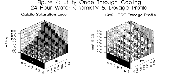
and continues to be demonstrated and optimized using online real time
control(2,3). Real time optimization is an economic necessity
in many of these lakes due to the high changes in pH encountered over even
a twenty four (24) hour period. pH fluctuations of 1.2 pH units have been
reported. As depicted in figure 4,
this equates to a ten fold change in dosage requirement in a single day.
Table 3 summarizes the water
chemistry, scale potential indices, and dosage recommendation for 100%
active HEDP for a single analysis and set of operating parameters for a
typical utility once through cooling system as outlined in one of the initial
dosage minimization studies(9). The treatment level recommended
is comparable to that found effective in the original published study.
It is of interest to note that the model which recommended an accurate
treatment level for a short residence time utility once through system
also recommends a reasonable treatment level for an open recirculating
cooling system with a residence time which can be calculated in days. The
model used for this comparison has been found to provide reasonable treatment
recommendations for both short and long residence time cooling systems.
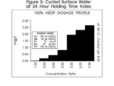
Figure 5 profiles a typical system.
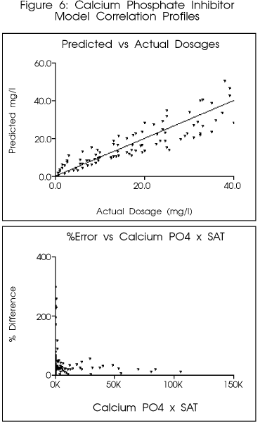
Example 2: Calcium phosphate Deposition Control
Calcium phosphate inhibitors have been successfully modeled by the
method described in the paper. The same basic formula was used for modelling
calcium phosphate deposition as was used for the calcium carbonate inhibitors.
Figure 6 indicates the preliminary
correlation for a copolymer in common use as a calcium phosphate inhibitor.
The model was applied to an open recirculating cooling system water chemistry
to determine if the dosages recommended were comparable to those effective
in operating systems. The treatment program had undergone extensive dosage
optimization to determine the most appropriate treatment level. The recirculating
water chemistry, operating parameters, and dosages for the system are outlined
in Table 4. The system typically
operates at approximately six (6) cycles of concentration.
The model predicted the final dosage within approximately ten (10) percent
of the final optimized value. Use of the model would have provided a reasonable
initial treatment level for the onsite optimization studies. An initial
dosage three times the optimized level was used as a starting point in
the actual study.
It is interesting to note that the coefficients calculated for the phosphonate
calcium carbonate inhibitors HEDP and AMP were of a comparable order, indicating
the same inhibition mechanism. The order for the calcium phosphate scale
inhibition by a copolymer is different, indicating a different scale inhibition
mechanism.
Summary
Laboratory and field dosage optimization data can be converted to a
mathematical model using standard statistical methods and a relationship
derived from theoretical models for induction time. The models provide
a practical method for collating laboratory and field data for a scale
inhibitor. The correlations developed can then be used to predict the dosage
for cooling systems based upon water chemistry and operating parameters
without the necessity for laboratory or indepth field studies to determine
the minimum effective dosage. Dosages predicted by models developed in
this manner are typically accurate as long as the system parameters and
water chemistry data are within the range of the data used to develop the
models. The examples presented in this paper are by necessity limited.
The basic models described in this paper have been used successfully in
systems ranging from short residence time, low scale potential systems,
to high residence time, high scale potential systems for calcium carbonate
control. The phosphate models have been used extensively as an integral
portion of treatment recommendation systems for multifunctional, alkaline
phosphate corrosion and scale control programs.
As with any predictive method, dosage recommendations from such models
should be evaluated by an experienced water treatment chemist prior to
implementation in an operational cooling system. Predicted dosages should
be used as a guideline, not as an ultimate treatment recommendation due
to factors which may not be taken into account by the models.
References
1. C.J. Schell, "The Use of Computer Modeling in Calguard
to Mathematically Simulate Cooling Water Systems and Retrieve Data,"
paper no. IWC8043 (Pittsburgh, PA: International Water Conference,
41rst Annual Meeting, 1980).
2. R.J. Ferguson, O. Codina, W. Rule, R. Baebel, "Real Time
Control of Scale Inhibitor Feed Rate," paper no. IWC8857
(Pittsburgh, PA: International Water Conference, 49th Annual Meeting, 1988).
3. S.R. Payne, B.W. Perrigo, R.M. Post, T.P. Clay, "Application
of a Selfcalibrating, Microprocessordriven Metering Device to
a Utility Once Through Cooling System," paper no. IWC9046
(Pittsburgh, PA: International Water Conference, 51rst Annual Meeting,
1990).
4. J.S. Gill, C.D. Anderson, R.G. Varsanik, "Mechanism of Scale
Inhibition by Phosphonates," paper no. IWC834 (Pittsburgh,
PA: International Water Conference, 44th Annual Meeting, 1983).
5. R.J. Ferguson, "Computerized Ion Association Model Profiles
Complete Range of Cooling System Parameters," paper no. IWC9147
(Pittsburgh, PA: International Water Conference, 52nd Annual Meeting, 1991).
6. R.J. Ferguson, "A Kinetic Model for Calcium Carbonate Deposition,"
CORROSION/84, Paper no. 120, (Houston, TX: National Association of Corrosion
Engineers, 1984).
7. R.J. Ferguson, "Practical Application of Condenser Performance
Monitoring to Water Treatment Decision Making," paper no. IWC8125
(Pittsburgh, PA: International Water Conference, 42nd Annual Meeting, 1981).
8. W.M. Hann, J. Natoli, "Acrylic Acid Polymers and Copolymers
as Deposit Control Agents in Alkaline Cooling Water Systems," CORROSION/84,
Paper no. 315, (Houston, TX: National Association of Corrosion Engineers,
1984).
9. B.W. Ferguson, R.J. Ferguson, "Sidestream Evaluation of Fouling
Factors in a Utility Surface Condenser," Journal of the Cooling Tower
Institute,2, (1981):p. 3139.
TABLE 1: MAJOR FACTORS INFLUENCING DOSAGE
| FACTOR |
IMPACT |
| Time |
Dosage increases with residence time. |
Degree of Supersaturation
|
Dosage increases with saturation level. |
| Temperature |
Dosage increases with temperature due to its impact upon
reaction rate.
This temperature impact is independent of any impact of temperature upon
saturation level. |
| pH |
Dosage may be pH dependent due to the impact of pH upon the
inhibitor dissociation state and stereochemistry.
This pH impact is independent of any impact of pH upon saturation level. |
| Suspended solids |
Dosage requirements may increase as suspended solids increase
due to absorbtion of the inhibitor on the solids.
|
| Active sites |
Dosage requirements increase if active sites for scale growth
are present.
It is easier to keep a clean system clean than it is to keep a dirty system
from getting dirtier.
|
TABLE 2: SATURATION LEVEL DEFINITION
Saturation level is the ratio of the Ion Activity
Product to the Solubility Product.
For calcium carbonate:
____________(Ca)(CO3)
______SL = _____________
______________Ksp'
For tricalcium phosphate:
___________(Ca)3(PO4)2
_____SL = _____________
_____________Ksp'
A water will tend to dissolve scale of the
compound if the saturation level is less than 1.0
A water is at equilibrium when the Saturation
Level is 1.0 . It will not tend to form or
dissolve scale.
A water will tend to form scale as the Saturation
Level increases above 1.0 .
Table 3: Utility Once Through Cooling
System Example
|
| Lake Water Analysis |
Deposition Potential Indicators |
| Cations |
Saturation Level |
| Calcium (as CaCO3) |
120.0 |
Calcite (CaCO3) |
3.94 |
| Magnesium (as CaCO3) |
34.0 |
Aragonite (CaCO3) |
3.84 |
| Sodium (as Na) |
14.00 |
Silica (SiO2) |
0.03 |
| Potassium (as K) |
0.00 |
Calcium phosphate (Ca3(PO4)2) |
0.00 |
| Iron (as Fe) |
0.10 |
Anhydrite (CaSO4) |
0.00 |
| Ammonia (as NH3) |
0.00 |
Gypsum (CaSO4 * 2H2O) |
0.00 |
| Aluminum (as Al) |
0.00 |
Fluorite (CaF2) |
0.00 |
| Boron (as B) |
0.00 |
Brucite (Mg(OH)2) |
0.01 |
| Anions |
Simple Indices |
| Chloride (as Cl) |
35.0 |
Langelier |
1.07 |
| Sulfate (as SO4) |
13.0 |
Ryznar |
6.27 |
| "M" Alkalinity (as CaCO3) |
120.0 |
Practical |
6.64 |
| "P" Alkalinity (as CaCO3) |
0.0 |
Larson-Skold |
0.39 |
| Silica (as SiO2) |
7.0 |
Treatment Recommendation |
| Phosphate (as PO4) |
0.0 |
10% HEDP (mg/L) |
0.20 |
| Fluoride (as F) |
0.0 |
Parameters |
| Nitrate (as NO3) |
0.0 |
pH |
8.40 |
| Other |
Temperature (oC) |
20.0 |
| Calculated TDS |
254 |
Residence Time (Seconds) |
5.60 |
Table 4: Calcium Phosphate Inhibitor
Dosage Optimization Example
|
| Lake Water Analysis |
Deposition Potential Indicators |
| Cations |
Saturation Level |
| Calcium (as CaCO3) |
1339. |
Calcite (CaCO3) |
38.77 |
| Magnesium (as CaCO3) |
496. |
Aragonite (CaCO3) |
32.90 |
| Sodium (as Na) |
1240. |
Silica (SiO2) |
0.39 |
| Potassium (as K) |
0.00 |
Calcium phosphate (Ca3(PO4)2) |
1,074. |
| Iron (as Fe) |
0.00 |
Anhydrite (CaSO4) |
1.33 |
| Ammonia (as NH3) |
0.00 |
Gypsum (CaSO4 * 2H2O) |
1.67 |
| Aluminum (as Al) |
0.00 |
Fluorite (CaF2) |
0.00 |
| Boron (as B) |
0.00 |
Brucite (Mg(OH)2) |
0.01 |
| Anions |
Simple Indices |
| Chloride (as Cl) |
620. |
Langelier |
1.99 |
| Sulfate (as SO4) |
3,384. |
Ryznar |
4.41 |
| Bicarbonate (as HCO3) |
294.1 |
Practical |
4.20 |
| Carbonate (as CO3) |
36.2 |
Larson-Skold |
0.39 |
| Silica (as SiO2) |
62.0 |
Treatment Recommendation |
| Phosphate (as PO4) |
6.20 |
100% Active Copolymer (mg/L) |
9.53 |
| Fluoride (as F) |
0.0 |
Parameters |
| Nitrate (as NO3) |
0.0 |
pH |
8.40 |
| Other |
Temperature (oC) |
20.0 |
| Calculated TDS |
609 |
Residence Time (Seconds) |
5.60 |